Mean, Median, and Mode of Grouped Data – Step-by-Step Lecture

Mean, Median, and Mode of Grouped Data: Complete Step-by-Step Guide

Understanding measures of central tendency—Mean, Median, and Mode—is fundamental to statistical analysis and quantitative research. When working with raw data organized into frequency tables and class intervals, individual data points are aggregated, requiring specific mathematical formulas for grouped data calculation.

SEO & Academic Focus:

Primary Keyword: Mean Median and Mode of Grouped Data
Target Level: Undergraduate & Graduate Statistics / Data Analysis
Key Topics: Frequency Distribution, Class Mark ($x$), Median Class Interpolation, Modal Class

The Example Dataset: Student Study Hours

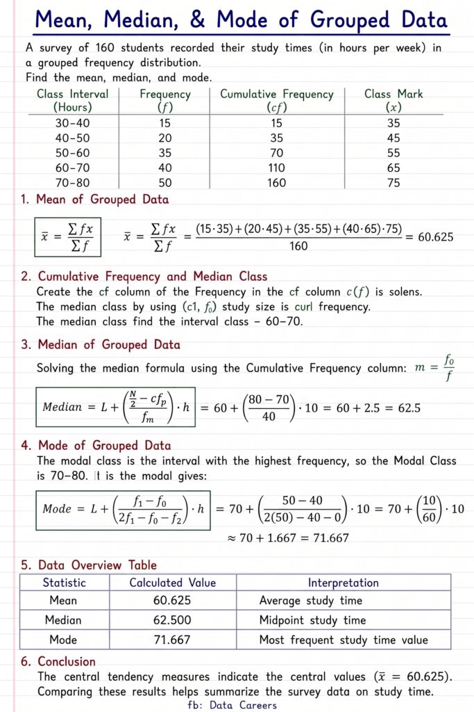
Consider a survey recording the weekly study hours of $N = 160$ students categorized into continuous class intervals:

Class Interval (Hours)	Frequency ($f$)	Class Mark / Midpoint ($x$)	Product ($f \cdot x$)	Cumulative Frequency ($cf$)
30 – 40	15	35	525	15
40 – 50	20	45	900	35
50 – 60	35	55	1,925	70
60 – 70	40	65	2,600	110
70 – 80	50	75	3,750	160
Total	$\sum f = 160$	—	$\sum fx = 9,700$	—

Class Width ($h$): $40 – 30 = 10$
Total Observations ($N$ or $\sum f$): $160$

1. Calculating the Mean ($\bar{x}$) of Grouped Data

The arithmetic mean represents the average or center of gravity of the distribution. Each class interval is represented by its class midpoint ($x$):

$$x = \frac{\text{Lower Limit} + \text{Upper Limit}}{2}$$

Mean Formula:

$$\bar{x} = \frac{\sum (f \cdot x)}{\sum f}$$

Step-by-Step Calculation:

Multiply each class frequency by its corresponding midpoint to get $f \cdot x$.
Sum all the products: $$\sum fx = 525 + 900 + 1,925 + 2,600 + 3,750 = 9,700$$
Divide by the total sample size ($N = 160$): $$\bar{x} = \frac{9,700}{160} = \mathbf{60.625 \text{ hours}}$$

2. Calculating the Median of Grouped Data

The median is the middle value dividing the distribution into two equal halves (50th percentile).

Step 1: Locate the Median Class

Find the median position using $\frac{N}{2}$:

$$\text{Position} = \frac{N}{2} = \frac{160}{2} = 80\text{th observation}$$

Referencing the Cumulative Frequency ($cf$) column, the 80th observation lies in the interval 60–70 (which covers values from 71 to 110).

Median Class: 60 – 70
Lower Boundary ($L$): 60
Cumulative Frequency preceding Median Class ($cf_p$): 70
Frequency of Median Class ($f_m$): 40
Class Width ($h$): 10

Median Formula & Computation:

$$\text{Median} = L + \left( \frac{\frac{N}{2} – cf_p}{f_m} \right) \cdot h$$

$$\text{Median} = 60 + \left( \frac{80 – 70}{40} \right) \cdot 10 = 60 + \left( \frac{10}{40} \right) \cdot 10 = 60 + 2.5 = \mathbf{62.50 \text{ hours}}$$

3. Calculating the Mode of Grouped Data

The mode identifies the point of highest frequency density in the dataset.

Step 1: Locate the Modal Class

The class interval with the highest frequency ($f = 50$) is 70–80.

Modal Class: 70 – 80
Lower Boundary ($L$): 70
Frequency of Modal Class ($f_1$): 50
Frequency of Preceding Class ($f_0$): 40
Frequency of Succeeding Class ($f_2$): 0 (terminal interval)
Class Width ($h$): 10

Mode Formula & Computation:

$$\text{Mode} = L + \left( \frac{f_1 – f_0}{2f_1 – f_0 – f_2} \right) \cdot h$$

$$\text{Mode} = 70 + \left( \frac{50 – 40}{2(50) – 40 – 0} \right) \cdot 10 = 70 + \left( \frac{10}{60} \right) \cdot 10 = 70 + 1.67 = \mathbf{71.67 \text{ hours}}$$

Summary of Results & Statistical Interpretation

Measure	Calculated Value	Statistical Interpretation
Mean ($\bar{x}$)	60.63 hrs	Arithmetic average study time per student.
Median	62.50 hrs	50% of students study < 62.50 hrs; 50% study > 62.50 hrs.
Mode	71.67 hrs	The most frequent study time cluster across the sample.

Distribution Skewness Insight:

Because $\text{Mean} < \text{Median} < \text{Mode}$ ($60.63 < 62.50 < 71.67$), the dataset is negatively skewed (left-skewed). This confirms that the majority of students are concentrated in higher study hour intervals, with fewer students logging low study hours pulling the mean downward.

Dr. Muhammad Asim Rafiq

Measure of Central Tendency