


Confidence Interval
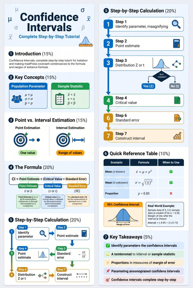
Confidence Intervals: Complete Step-by-Step Tutorial on Point and Interval Estimation
1. Learning Objectives
By the end of this lecture, students should be able to:
- Understand point estimation and interval estimation
- Distinguish between a parameter, statistic, and estimator
- Calculate point estimates for a population mean and proportion
- Construct confidence intervals for a population mean
- Decide when to use Z and t distributions
- Construct a confidence interval for a population proportion
- Interpret confidence intervals correctly
- Calculate the margin of error
- Determine the required sample size for estimating a mean or proportion
- Understand the effect of sample size and confidence level on interval width
2. What Is Estimation?
In statistics, we usually want to learn something about a population, but collecting data from the entire population is often impossible.
For example, suppose a university has 10,000 students and we want to know their average monthly expenditure.
We cannot necessarily survey all 10,000 students.
Instead, we select a sample, for example:
students.
We then use the sample information to estimate the population parameter.
The process is called statistical estimation.
There are two major types:
- Point estimation
- Interval estimation
3. Parameter vs. Statistic
This distinction is extremely important.
Population Parameter
A parameter describes the population.
Examples:
Usually, the parameter is unknown.
Sample Statistic
A statistic describes the sample.
Examples:
We use these sample statistics to estimate unknown population parameters.
4. Point Estimation
Definition
A point estimate is a single numerical value used to estimate an unknown population parameter.
For example, suppose we want to estimate the average income of a population.
We take a sample and obtain:
Our point estimate of the population mean is:
We are using one number to estimate the unknown population mean.
5. Common Point Estimators
| Population Parameter | Point Estimator |
|---|---|
| Population mean (μ) | Sample mean (x̄) |
| Population proportion (p) | Sample proportion (p̂) |
| Population variance (σ²) | Sample variance (s²) |
| Population standard deviation (σ) | Sample SD (s) |
For today’s lecture, the most important are:
6. Example 1: Point Estimate of a Population Mean
Suppose a researcher selects 8 students and records their weekly study hours:
Step 1: Calculate the sample mean
The total is:
Therefore:
Answer
The point estimate of the population’s average weekly study time is:
Notice that we do not know the actual population mean.
We are using:
as our estimate.
7. Why Is a Point Estimate Not Enough?
Suppose Student A takes a sample of 100 students and obtains:
Student B takes another sample of 100 students and obtains:
Student C obtains:
Which value is the true population mean?
We do not know.
A point estimate provides one best estimate, but it does not tell us how much uncertainty surrounds that estimate.
This is why we need interval estimation.
8. Interval Estimation
Instead of giving one value, we provide a range of plausible values for the population parameter.
For example:
This is an interval estimate.
A confidence interval normally has the form:
Therefore:
This is the central idea behind confidence intervals.
9. What Is a Confidence Interval?
A confidence interval (CI) is a range of values calculated from sample data that is designed to capture an unknown population parameter with a specified level of confidence.
Common confidence levels are:
- 90%
- 95%
- 99%
The most commonly used level is:
10. The Basic Structure of a Confidence Interval
Every confidence interval can be understood as:
Therefore:
where:
So the calculation has three major components:
1. Point estimate
What is our best estimate?
2. Standard error
How much sampling variability exists?
3. Critical value
How much uncertainty do we want to cover?
11. Confidence Level and Critical Values
For the standard normal distribution:
| Confidence Level | Critical Value (zα/2) |
|---|---|
| 90% | 1.645 |
| 95% | 1.960 |
| 99% | 2.576 |
For example, at 95% confidence:
12. Why Do We Use α?
If the confidence level is 95%:
The remaining probability is:
Because the interval is two-sided, this 5% is divided between the two tails:
Therefore:
This gives the familiar 95% confidence interval.
13. Confidence Interval for a Population Mean
There are two important cases.
Case 1: Population standard deviation (σ) is known
Use the Z distribution:
Case 2: Population standard deviation (σ) is unknown
Use the t distribution:
where:
- x̄ = sample mean
- σ = population standard deviation
- s = sample standard deviation
- n = sample size
- zα/2 = Z critical value
- tα/2, n−1 = t critical value
- n − 1 = degrees of freedom
14. Example 2: 95% Confidence Interval When σ Is Known
Suppose:
Construct a 95% confidence interval for the population mean.
Step 1: Identify the information
Confidence level: 95%
Since σ is known, we use the Z distribution.
Step 2: Find the critical value
For 95% confidence:
Step 3: Calculate the standard error
Step 4: Calculate the margin of error
Step 5: Calculate the confidence interval
Lower limit: 72 − 2.45 = 69.55
Upper limit: 72 + 2.45 = 74.45
15. Example 3: Confidence Interval When σ Is Unknown
Suppose a researcher studies the monthly spending of 25 students.
The results are:
Construct a 95% confidence interval for the population mean.
Step 1: Determine whether to use Z or t
The population standard deviation is unknown.
We have: s = 12
Therefore, use the t distribution.
Step 2: Calculate degrees of freedom
Step 3: Find the critical t-value
For 95% confidence and df = 24, the critical value is approximately:
Step 4: Calculate the standard error
Step 5: Calculate the margin of error
Step 6: Calculate the confidence interval
Lower limit: 68 − 4.95 = 63.05
Upper limit: 68 + 4.95 = 72.95
16. Z vs. t: What Should Students Remember?
Use this simple decision process:
For the standard one-sample mean problem, when σ is unknown, the t-distribution is the appropriate choice.
The t-distribution has heavier tails than the standard normal distribution, reflecting the additional uncertainty from estimating σ using s.
17. Confidence Interval for a Population Proportion
Suppose the population parameter of interest is a proportion:
The sample proportion is:
where:
- x = number of successes
- n = sample size
The approximate confidence interval is:
18. Example 4: Confidence Interval for a Proportion
Suppose a university surveys 200 students.
Out of 200 students, 120 say that they prefer online learning.
Find the 95% confidence interval for the population proportion.
Step 1: Calculate the sample proportion
Therefore, 60% of the sample prefers online learning.
Step 2: Find the critical value
For 95% confidence:
Step 3: Calculate the standard error
Step 4: Calculate the margin of error
Step 5: Calculate the confidence interval
Lower limit: 0.60 − 0.06790 = 0.53210
Upper limit: 0.60 + 0.06790 = 0.66790
In percentage terms:
19. Complete Confidence Interval Formula Sheet
Population Mean — σ Known
Population Mean — σ Unknown
Population Proportion
20. Margin of Error
The margin of error (ME) tells us how far the confidence interval extends on either side of the point estimate.
Generally:
For a mean with known σ:
For a mean with unknown σ:

Post navigation
Previous Post
 Central Limit Theorem